
Cheetah documentation - all keywords
Data Analysis
This resource belongs to the Data Analysis group.
Category
Published on
Abstract
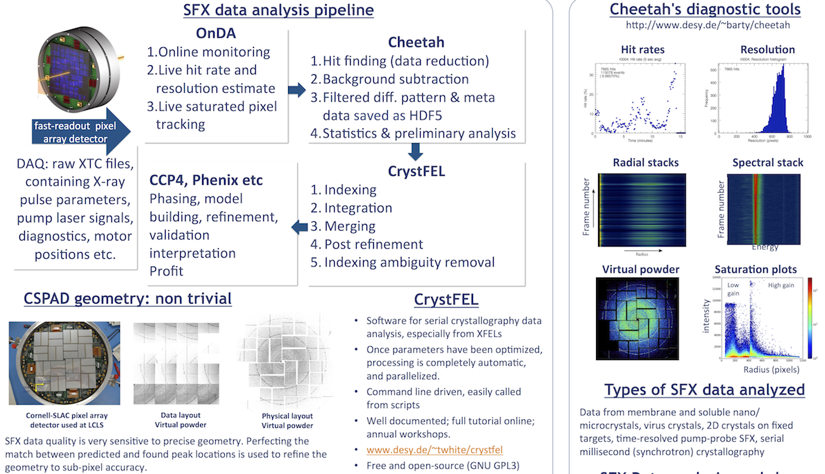
The official Cheetah website is http://www.desy.de/~barty/cheetah/
These pages will not reproduce all the content from the Cheetah site, but are meant as an addendum.
Complete listing of keywords for Cheetah's configuration files
Many of these are power user settings designed for turning on or off features in testing.
Detector configuration
detectorName (CxiDs1)
Recognized options for cspad are:
- "CxiDs1": CSPAD,
- typically in position DsC, “front detector” in 1 µm chamber at CXI
- "CxiDs2": CSPAD
- typically in position DsD, i.e. “back detector” in 1 µm chamber at CXI, downstream of Ds1
- "XppGon": cspad on XPP beamline
CxiDs1 is the name of the CSPAD (Cornell SLAC pixel array detector). Talk to your beamline scientist to confirm.
geometry (geometry/cspad_pixelmap.h5)
Path to an hdf5 file specifying the real-space coordinates of each pixel. The hdf5 data fields are /x /y and /z. The x coordinate corresponds to data fast scan coordinates (pixels that are nearest neighbors in memory), while y is slow scan. The z coordinate is the relative offsets of each detector panel. Units are meters (values are first divided by pixel size variable to get coordinates of pixels in space).
Note: see the keyword pixelSize-- it is important that this is consistent with the units in the geometry!
pixelSize (0.000110)
Size of pixels in meters, defaults to values for the CSPAD detector (110 µm).
defaultcameraLengthmm (100)
The default camera length (in mm) to use in the event that the detector position encoder value is not available in the XTC data stream.
cameraLengthOffset (592.0)
Offset (in mm) to add to value from detectorZpvname to get absolute sample-detector distance.
cameraLengthScale (0)
defaultphotonenergyev
The default photon energy (in eV) to use in the event that the beamline data is not available in the XTC data stream.
detectorZpvname (CXI:DS1:MMS:06.RBV)
The LCLS EPICS process variable name needed for accessing the encoder value for the camera length of the detector in position DS1. This is the front detector encoder value for experiments in the 1 µm chamber.
- DSA for the position immediately after the SC01 (aka SC2) chamber for the 100nm focus.
- DSB for the position in front of the SC1 chamber
- DSC for the front detector position immediately after the SC1 chamber (1 µm focus)
- DSD for the back detector position
DS[0-9] are the CSPAD labels, DS[A-Z] are CSPAD locations. Typically, we expect to have the following configuration:
- DS2 in the DSC location
- DS1 in the DSD location
Calibration and masks
darkcal (darkcal.h5)
Path to an input hdf5 file containing a dark current measurement. Cheetah can create a "darkcal" from a dark run; see the generateDarkcal keyword. The hdf5 data field is "/data/data". Units are ADU. Darkcals should NOT be gain corrected.
Make sure the detector gain settings of the darkcal match that of the run.
gaincal (gaincal.h5)
Path to an input hdf5 file containing the gainmap. By default the raw data will be multiplied by this map, although it can be inverted by setting invertGain=1. The hdf5 data field is "/data/data".
invertGain (0)
Divide by the gain map, rather than multiplying (in case gain map is supplied as gain per pixel, rather than value to multiply pixel values by).
peakMask (peakmask.h5)
Path to an input hdf5 file indicating where not to search for peaks, but without masking out the region which “badpixelmap” does. The hdf5 data field is "/data/data".
badPixelmap (badpixels.h5)
Path to input hdf5 file indicating bad pixels which will be masked in clean hdf5’s. Essentially, this has the same effect as a gainmap. The hdf5 data field is "/data/data"
Cheetah’s GUI can generate a bad pixel map automatically from the darkcal.h5. See step 4 on http://www.desy.de/~barty/cheetah/Cheetah/Cheetah_at_LCLS.html
savePixelMask (1)
Save a copy of the pixel mask as badpixelmap.h5 in the HDF5 directory.
maskSaturatedPixels (0)
Search each image for saturated pixels, and mask them prior to further analysis. Saturated pixels are identified by a simple global threshold value set by the keyword pixelSaturationADC.
Background subtraction
Proper subtraction of electronic and photon background is essential – there are many options.
# Unbonded pixels only for cspad v1.6 modules (January 2014 onwards)
# commonModeCorrection = {none, asic_histogram, asic_median, asic_unbonded}
One of three possible methods for subtracting common mode offsets from individual ASICs.
Common mode noise on each ASIC fluctuates randomly from frame to frame and must be estimated from the read out signal itself. Common mode is estimated as the lowest 10% of pixel values in each ASIC. 10% value can be set to something else by the user if desired.
This option assumes the lowest 10% of values represent only detector electronic noise - be careful of using this when there are no dark areas on the ASIC.
Pixel locations are hard coded for testing (generalize later)
subtractUnbondedPixels (0)
cmFloor (0.100000)
Use lowest x% of values as the offset to subtract (typically lowest 2%)
useAutoHotpixel (0)
Automatically identify and remove hot pixels. Hot pixels are identified by searching for pixels with intensities consitently above the threshold set by the keyword hotpixADC. In this case, "consistently" means that a certain fraction (user-set keyword hotpixFreq) of a certain number of buffered frames (number of frames set by the keyword hotpixMemory) are above threshold. The hot pixel map is updated every hotpixMemory frames.
Hot pixels within the corrected data will be set to zero. Note that the search for hot pixels is performed on the correcteddata (probably it should be performed on raw data instead?), so if you decide to change the corrections (e.g. darkcal, gainmap), the resulting hot pixel maps may differ.
useSubtractPersistentBackground (0)
Subtract the pixel-by-pixel median background calculated from the previous N frames (N set by the keyword bgRecalc, but apparently it cannot exceed 50 frames – it can, if bgbuffer is made large enough).
useLocalBackgroundSubtraction (0)
Prior to peak searching, transform the image by subtracting the median value of nearby pixels. The median is calculated from a box surrounding each pixel. The size of the box is equal to localBackgroundRadius*2 + 1
Bad pixels and detector edge effects are not accounted for (i.e., if most nearby pixels are bad, the local median will be equal to zero). This is somewhat slower, but very effective for nanocrystal data.
localBackgroundRadius (3)
See keyword useLocalBackgroundSubtraction.
Background calculation tuning
bgMemory (50)
See keyword useSubtractPersistentBackground.
bgRecalc (50)
Strange, this *almost* does the same thing as bgMemory, butif bgRecalc is less than the default value of bgMemory, that default value will be used?
This sets how often the program pauses to recalculate background and hot pixel values. It is typically the same as the buffer size, but since recalculation is a thread blocking process, setting this to happen less frequently (eg: every 200 or 500 frames) speeds up execution.
bgMedian (0.5)
Rather than using the usual median value for background, you can optionally choose any arbitrary K-th smallest element equal to bgMedian*bgMemory. Neat!
bgIncludeHits (0)
Include hits in the background running buffer.
bgNoBeamReset (0)
Used to reset the background buffer whenever LCLS beam dies, defined as when GMD<0.2mJ. (not implemented)
bgFiducialGlitchReset (0)
Used to restart backgrounds when LCLS unexpected changes operating frequency. This was a problem on hot days in the June 2010 data set. (not implemented)
Automatic hot pixel calculation
hotpixFreq (0.9)
See keyword useAutoHotPixel.
hotpixADC (10000)
See keyword useAutoHotPixel.
hotpixMemory (50)
See keyword useAutoHotPixel.
Pixel saturation
maskSaturatedPixels (0)
Search each image for saturated pixels, and mask them prior to further analysis. Saturated pixels are identified by a simple global threshold value set by the keyword pixelSaturationADC.
pixelSaturationADC (65535)
See keyword maskSaturatedPixels.
Hit finding algorithms
hitfinder (0)
Specify the hitfinder algorithm. Various flavours of hitfinder:
- Number of pixels above ADC threshold
- Total intensity above ADC threshold
- Count Bragg peaks (intensity threshold)
- Use TOF
- Count Bragg peaks (threshold + gradient + extras)
- Count Bragg peaks (based on signal-to-noise ratio)
- Count Bragg peaks (based on signal-to-noise ratio with radial background averaging)
Note that the choice of hitfinder influences what is reported in the log files.
First, do these steps (regardless of the hitfinder choice): Build a buffer, which is a replica of the corrected data. Values in the buffer array will be set to zero as those pixels are analyzed and rejected. If hitfinderUsePeakmask != 0, then multiply the buffer by this array before moving on.
Now, depending on the algorithm, do these steps:
Algorithm 1:
- Count the pixels within the buffer that are above the (user-defined) hitfinderadc value.
- Also, sum the values of the pixels that meet the criteria of step 1.
- If the number of pixels is greater than the value of (user-defined) hitfindernat, count this frame as a hit.
- Report the number of pixels in the log files as npeaks and as nPixels.
- Report the total counts (intensity) as peakTotal
Algorithm 2:
Same as algorithm 1, except that the criteria for a hit is now that the *intensity* is greater than hitfindernat, rather than the pixel count.
Algorithm 3:
Briefly, this is what happens:
- Scan the buffer, module-by-module, searching for "blobs" of connected pixels which all meet the criteria of being above the threshold defined by the keyword hitfinderADC. A pixel can be "connected" to any of its eight nearest neighbors. If its "connected" neighbor is "connected" to another pixel, then all three are mutually "connected" to each other.
- If a blob contains more than hitfinderMinPixCount connected pixels, and less than hitfinderMaxPixCount pixels, it is counted as a peak.
- The center of mass and integrated intensity is calculated for the blob (this is the peak position and integrated intensity).
- If there are more than hitfinderNpeaks peaks, and less than hitfinderNpeaksMax, then count this as a hit.
Some important keywords:
- hitfinderNAT
- hitfinderADC
- hitfinderMinPixCount
- hitfinderMaxPixCount
- hitfinderNPeaks
- hitfinderNPeaksMax
- hitfinderCheckMinGradient: Before considering a peak candidate, check that the intensity gradient is above this threshold. Here, the "gradient" is the mean square derivative of the "above/below" and "upper/lower" pairs of pixels connnected to the pixel of interest.
- hitfinderMinGradient: Threshold for the above keyword.
- hitfinderCheckPeakSeparation: After locating peaks, throw out all the peak pairs that are too close together.
- hitfinderMaxPeakSeparation: Threshold for the above keyword.
This algorithm also calculates a quantity called "peak density".
Algorithm 4:
Use time-of-flight data. Detail coming soon.
Algorithm 5:
Similar to 3. Details coming soon.
Algorithm 6:
Firstly, create a combined mask which indicates hot pixels, saturated pixels, bad pixels, pixels specifically masked at the peakfinding stage (keyword peakmask), and pixels outside the specified resolution range (keywords hitfinderLimitRes, hitfinderMinRes, hitfinderMaxRes). These pixels will never be considered for further analysis.
Each pixel in each detector panel (one panel at a time) will be inspected. Initially, we are seaching for a simple "trigger" to indicate the possibility of a peak, with more stringent tests to follow. Here's how it works:
- If the pixel intensity (in raw ADC units) is below the threshold set by hitfinderADC, skip this pixel.
- If any of the eight nearest neighbor pixels has a greater intensity, skip this pixel.
- If the above tests pass, the signal-to-noise ratio (SNR) will be calculated as follows: the mean background intensity <I> and the standard deviation sig(I) are calculated from a concentric square annulus, with its radius specified by the keyword hitfinderLocalBGRadius. The thickness of the annulus is specified by the keyword hitfinderLocalBGThickness. (For example, if the radius is 1, and the thickness is 1, then only the nearest 8 pixels will be considered in this calculation.) The SNR for this pixel is equal to (I-<I>)/sig(I).
- If the background-corrected intensity (I - <I>) is less than the threshold hitfinderADC, skip this pixel.
- If the SNR value is below the value hitfinderMinSNR, skip this pixel.
- If the above tests pass, a test for how many connected pixels also meet the above criteria will be performed. If the number of connected pixels falls within the (inclusive) range [ hitfinderMinPixCount , hitfinderMaxPixCount ], then this will be counted as a peak. Note that connected pixels are masked, and will not be considered for further analysis.
- The centroid of the peak will be calculated (within the box of radius equal to hitfinderLocalBGRadius).
- Once a peak is found, a test will be performed to check that there are not other peaks that are too close to this one. The limiting distance is set by the keyword hitfinderMaxPeakSeparation. If a closer peak is found, it will be eliminated if it has lower SNR than this peak, else the current peak will be eliminated. (Note that, currently, this does not guarantee that some closely-spaced peak pairs will not be found, but will eliminate most of them).
- Once the last pixel has been analyzed, if the number of peaks found is in the (inclusive) range [ hitfinderMinPeaks, hitfinderMaxPeaks ], then this pattern will be considered a hit.
Algorithm 7:
Coming soon.
Algorithm 8:
This is now the most commonly used hit finding algorithm for serial crystallography experiments.
This algorithm uses a radial average to determine the SNR and intensity threshold. If there are shadows in your patterns, be sure to mask these regions during peak finding by using a PeakMask (see peakmask section above).
Some important keywords:
- MinADC
- MinSNR
- Npeaks
- NpeaksMax
- MinPixCount
- MaxPixCount
- LocalBgRadius
- MinPeakSeparation
- MinRes
- MaxRes
- FastScan
Hitfinder tuning
hitfinderAlgorithm (8)
See the keyword hitfinder.
hitfinderADC (100)
See the keyword hitfinder.
hitfinderNAT (100)
See the keyword hitfinder.
hitfinderNPeaks (50)
See the keyword hitfinder.
hitfinderNPeaksMax (100000)
See the keyword hitfinder.
hitfinderMinPixCount (3)
See the keyword hitfinder.
hitfinderMaxPixCount (20)
See the keyword hitfinder.
hitfinderLocalBGRadius (4)
See the keyword hitfinder.
hitfinderLocalBGThickness (1)
See the keyword hitfinder.
hitfinderLimitRes (0)
See the keyword hitfinder.
hitfinderMinRes (0)
See the keyword hitfinder.
hitfinderMaxRes (0)
See the keyword hitfinder.
For weak diffraction spots, it may help to restrict the search for spots to within the diffuse ring from water, LCP etc, to avoid picking up false peaks. However, note that limiting the peak finding resolution impacts on geometry refinement and both of CrystFEL’s resolution prediction and integration radius refinement)
hitfinderUseTof (0)
Does choosing hitfinding algorithm 4 accomplish the same thing?
hitfinderTofMinSample (0)
?
hitfinderTofMaxSample (1000)
?
hitfinderTofThresh=1283604304
?
Specifying what gets saved in exported frame HDF5 files
saveCXI (1)
As of February 2015 the default file format changed from individual HDF5’s to CXIDB format (www.cxidb.org). A description of the .cxi format for multi-event data collected on a CSPAD at LCLS can be found at the bottom of this document or on the CXIDB website. In summary – all hits and metadata are stored in a single HDF5. This format is compatible with the Cheetah GUI and the online data analysis software OnDA.
To generate many small HDF5’s, set saveCXI to 0 (this is the original approach).
saveHits (0)
Save the hits to individual hdf5 files. Exactly what will be saved is determined by the keywords saveRaw, saveAssembled, savePeakInfo, saveDetectorCorrectedOnly, saveDetectorRaw, and possibly more...
saveNonAssembled (1)
Save detector data as hdf5 without geometry corrections, i.e. in the layout as read from the detector, without interpolation into a physically realistic image.
saveAssembled (1)
Save the data after it has been interpolated into a physically correct image (as would be seen on a sheet of film), based on the geometry file. Note that this will take up more space on disk, but provides an image that can be analysed/displayed as if the detector were one CCD. Also, note that geometry is updated sometimes, and you will need to re-run all of your hit finding if you intend to store the data only in assembled form (not recommended). The hdf5 field is /data/assembleddata, and has zeros where there is no data. If present, it will be symbolically linked to the field /data/data.
saveDetectorRaw (0)
Save detector data as hdf5 without photon corrections, i.e. no dark current subtraction and no other background subtraction or masks applied.
saveDetectorCorrected (1)
Save detector data in the hdf5 files with dark current subtraction, gain calibration (if gaincal is specified), and bad pixel mask applied. This does not include further background subtraction, nor does it involve geometry in any way.
This is the recommended option. Even if background subtraction is used for hit finding, back up to image with only detector corrections subtracted and save this instead. Useful for preserving the water ring, for example.
If set to non-zero value, save the data which has only the following operations done to it (in this order):
- Subtract darkcal
- Subtract common mode offsets
- Apply gain correction
- Multiply by bad pixel mask
If set to zero, then you get these additional corrections (in this order):
- Subtract running (persistent) background
- Subtract local background
- Zero out hot pixels
- Multiply by bad pixel mask (again)
If the keyword saveDetectorRaw is set, then none of the above corrections will be applied (therefore, this keyword has no effect).
saveDetectorAndPhotonCorrected (0)
Same as saveDetectorCorrected = 1 followed by background subtraction.
If set to 1, save the data which has the following operations done to it (in this order):
- Subtract darkcal
- Subtract common mode offsets
- Apply gain correction
- Multiply by bad pixel mask
- Subtract running (persistent) background
- Subtract local background
- Zero out hot pixels
- Multiply by bad pixel mask (again)
If the keyword saveDetectorRaw is set, then no corrections will be applied (i.e. this keyword will have no effect).
saveDetectorRaw (0)
Image will be saved exactly as represented in the XTC data stream (even before dark current subtraction), regardless of what detector corrections and photon background subtraction is used for hit finding. This option is mainly of interest to detector groups who want to look at data in as raw a form as possible, or for low-level diagnostics on common mode, electronic noise, etc.
This keyword trumps the keywords saveDetectorCorrected and saveDetectorAndPhotonCorrected.
hdf5dump (0)
Write every nth frame to an hdf5 file, regardless of whether it was found to be a hit.
dataSaveFormat (INT16)
Accepted formats = INT16, INT32, float.
saveEpicsPVfloat (no default)
What EPICS process variables you want saved to the .cxi format output, up to 99 entries. Not available if saveCXI=0
E.g. saveEpicsPVfloat=CXI:TTSPEC:FLTPOS
saveEpicsPVfloat=CXI:LAS:MMN:06.RBV
Creation of calibration files
generateDarkcal (0)
Create a darkcal from a given run (which should contain dark data -- i.e. data without the X-ray beam on). Takes the average of all patterns, and output a "darkcal" hdf5 file named rXXXX-darkcal.h5 in the end. Essentially, this option tricks cheetah into thinking every frame is a "hit". The darkcal is the average, not the sum, unlike the usual "powder" patterns. If you set generatedarkcal=1, the following keywords will be modified so everything works as expected:
- cmModule = 0;
- cmSubtractUnbondedPixels = 0;
- subtractBg = 0;
- useDarkcalSubtraction = 0;
- useGaincal=0;
- useAutoHotpixel = 0;
- useSubtractPersistentBackground = 0;
- hitfinder = 0;
- savehits = 0;
- hdf5dump = 0;
- saveRaw = 0;
- saveDetectorRaw = 1;
- powderSumHits = 0;
- powderSumBlanks = 0;
- powderthresh = -30000;
- startFrames = 0;
- saveDetectorCorrectedOnly = 1;
generateGaincal (0)
Automatically create a gain map file from flat field data. Works, but the output likely needs tweaking by hand in IDL/Matlab. All patterns will be summed to form an average, which is then divided by the median value of the image. (The median value is therefore gain = 1.) The gainmap will be saved as "rXXXX-gaincal.h5". At the moment, the gainmap is set to zero where it is outside of the bounds 0.1 and 10. When setting generategaincal=1 the following keywords will be modified so everything works as expected:
- cmModule = 0;
- cmSubtractUnbondedPixels = 0;
- subtractBg = 0;
- useDarkcalSubtraction = 1;
- useAutoHotpixel = 0;
- useSubtractPersistentBackground = 0;
- useGaincal=0;
- hitfinder = 0;
- savehits = 0;
- hdf5dump = 0;
- saveRaw = 0;
- saveDetectorRaw = 1;
- powderSumHits = 0;
- powderSumBlanks = 0;
- powderthresh = -30000;
- startFrames = 0;
- saveDetectorCorrectedOnly = 1;
Image summation (powder patterns)
powderSumHits (1)
Record and save the summed (not averaged) intensities from frames determined to be hits. Will be saved as the file named rXXXX-detector0-class1-sum.h5 where XXXX is the run number (e.g. 0013). The hdf5 data field is /data/data.
powderSumBlanks (1)
Record and save the summed (not averaged) intensities from frames determined to be non-hits. Will be saved as the file named powderSumBlanks.h5. The HDF5 data field is /data/data.
powderThresh (-20000)
Apply this intensity threshold before powder summation. Setting to ~500 typically captures only peaks; setting to 0 sums only positive values; setting to -20,000 typically sums everything.
savePowderDetectorRaw (0)
Apply this intensity threshold before powder summation. Setting to ~500 typically captures only peaks; setting to 0 sums
savePowderDetectorCorrected (1)
Same steps as “saveDetectorCorrected” applied to summed intensities. HDF5 dataset is /data/non_assembled_detector_corrected, linked to from /data/data and /data/correcteddata. A dataset of the detector corrected pixels’ sigma is also recorded, in /data/non_assembled_detector_corrected_sigma
savePowderDetectorAndPhotonCorrected (1)
Same as savePowderDetectorCorrected = 1, followed by background subtraction. HDF5 dataset is /data/non_assembled_detector_and_photon_corrected. A dataset of the detector and photon corrected pixels’ sigma is also recorded, in /data/non_assembled_detector_and_photon_corrected_sigma
savePowderNonAssembled (1)
Save the summed detector data as hdf5 without photon or geometry corrections, i.e. in in data layout as read from the detector, without interpolation into a physically realistic image.
savePowderAssembled (0)
Save the summed (not averaged) intensities which has been interpolated into a physically correct image (as would be seen on a sheet of film), based on the geometry file.
The hdf5 field is /data/assembleddata, and has zeros where there is no data. If present, it will be symbolically linked to the field /data/data.
usePolarizationCorrection (0)
Radial intensity profiles (SAXS/WAXS profiles)
saveRadialStacks (0)
Save hdf5 files containing radial profiles, image-by-image. Masked pixels will not be integrated. More details here some day.
radialStackSize (10000)
How many radial profiles in each hdf5 "radial stack" file.
Energy spectrum
espectrum (0)
Toggles the creation of a 2D array from the readout of the energy spectrum CCD.
espectrum1D (1)
Toggles the creation of a 1D line output of the beam energy profile, calculated by integration of the energy spectrum CCD along the line of the stripes in the spectral profile.
Toggles the removal of a mean background from the CCD before calculation of the 1D integrated spectrum. A background is calculated when the generateDarkcal flag is set to 1
espectrumTiltAng (0)
Input which specifies the tilt of the spectral stripes with respect to the horizontal axis of the CCD. The angle is defined so that a positive value relates to a clockwise rotation of the spectral stripes from the horizontal. This can be calculated from the first run of the experiment from an image of the spectrum CCD camera in the event hdf5 file in the field “/data/espectrumCCD”. This value is likely to change if the spectrum CCD is moved, i.e. in the event of an energy change or X-ray beam re-focusing.
espectrumLength (1080)
Number of pixels along the energy axis of the spectrum CCD camera. Defaults to the value for the long axis of an Opal2K CCD of 1080 pixels
espectrumWidth (900)
Number of pixels along the beam profile axis of the spectrum CCD camera. Defaults to the value for the short axis of an opal2K CCD of 900 pixels
espectrumSpreadeV (40)
Value of the energy spread seen by the energy spectrum CCD camera in eV. Defaults to 40
espectrumDarkfile ()
Path to the energy spectrum dark calibration file created from a dark calibration run. The filename will have the format rXXXX-energySpectrum-darkcal.h5. If the espectrumDarkSubtract keyword is set to 1 and no file path is given or the specified file does not exist the program will terminate.
espectrumScalefile (0s)
Path to a file which is used in an attempt to calibrate the spectral profile to absolute energy values. At the end of each run a spectrum integrated over the whole run is calculated, the maximum in this run-integrated spectrum is assigned the average beam energy value (as reported by global->meanPhotonEnergyeV). A scale is generated based on the known energy spread of the spectrum CCD and saved in the rXXXX-integratedEnergySpectrum.h5 file. The scale can be assigned to individual events by either re-running cheetah with the scale file belonging to that run or the scale from a previous run can be applied. If no file is given or the file specified does not exist the individual event spectra are output with zeros for the energy scale (the program does not terminate)
Time of flight spectrometer (Acqiris)
tofName (CxiSc1)
Can be use for pump laser diode trace?
tofName (CxiSc1)
Name of Acqiris device in XTC data stream
tofChannel (1)
Acqiris channel number
Multithread tuning and speed optimization
nThreads (16)
Run this many worker threads in parallel (one worker thread per LCLS event). Set to 1x-2x the number of cores on the machine.
- 72 or 144 on cfelsgi (72 physical cores)
- 16 is more than adequate on most servers (eg: compute farm at SLAC uses 12 or 16 core machines)
Speed may saturate before all threads are busy if data transfer makes cheetah I/O limited (check with ipSpeedTest), or if competing access to shared variables results in mutex locks (happens when too many threads write to powder patterns or running background buffer at once).
useHelperThreads (0)
Inactive keyword. It was intended for computing backgrounds asynchronously with processing data frames.
saveInterval (1000)
Periodically save running sums and update the log file at this interval.
Data processing flow: skipping XTC frames
startAtFrame (0)
Skip all frames in the xtc file prior to this one (no processing done).
stopAtFrame (0)
Skip all frames in the xtc file after this one. Setting to 0 means to ignore this setting.
startFrames (0)
Number of frames at the start of processing used for background estimates, etc, before starting hit finding etc.
ioSpeedTest (0)
Run through events in xtc file, reading in all data, but do no data processing (don't spawn worker threads). Useful for checking raw I/O speed to determine whether the process is I/O bound or CPU/mutex bound.
Time resolved work
sortPumpLaserOn (0)
Sort data into classes based on pump laser signal. See pumpLaserScheme.
pumpLaserScheme (evr41)
What scheme of sorting by pump laser (probe) to use for separating time-resolved data. Options: evr41, LD57,
More schemes will be added in the future. This string is used to toggle the information fed into laserOn and the way in which patterns are sorted. Places that need changing if this ever changes are: (a) what is in laserOn, (b) setting the number of powder pattern, (c) setting the powder class.
saveByPowderClass (1)
laserOn can be more than on or off. Let this be 0,1 or 2 depending on which laser is on. This scales in many ways e.g.: it can be a simple number of a binary mask if multiple lasers are on at once.
Misc
debuglevel (2)
Sets verbosity level of the output (how much diagnostic junk is printed to screen)
useFEEspectrum (0)
Used for diagnostic purposes
References
Click here for Cheetah documentation (main)
Click here for Cheetah documentation (page 1)
Click here for Cheetah documentation (page 2)
Back to front page: LCLS serial femtosecond crystallography data analysis instructions


